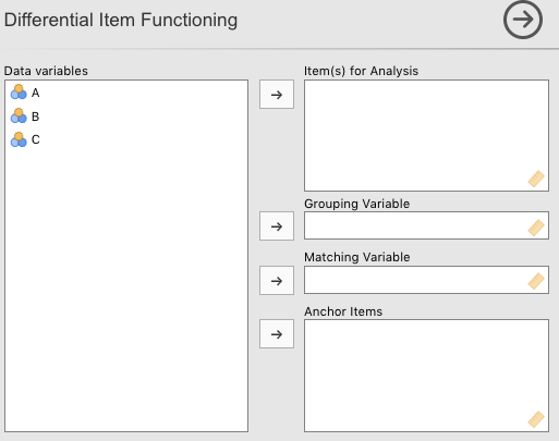
1. Items

Items must be a series (vector) of names referencing columns in the data containing exactly two unique values, such as [0, 1]. The data will be converted to integer type prior to analysis using jmvcore::toNumeric().

2. Grouping Variable

Grouping Variable must be a single name referencing a column in the data containing at least two unique values, such as [0, 1]. The data will be converted to factor type prior to analysis using base:as.factor().

The value of the first row in the column will be coded as Group A, and all rows containing non-Group A values will be coded as Group B. If more than two unique values are present in the column, all values different from the value of the first row will be collapsed into the same Group B. This restriction will be removed in a future version of the module, but is necessary for several aspects of the current version to perform.

3. Matching Variable

Matching Variable is an optional argument. This is the value which is used in the regression equations to account for differences in, for example, proficiency, levels of a latent contstruct, or some other psychosocial factor. If it is left empty, subjects will be matched on the Total Score, calculated internally by the module. This variable must be numeric.

4. Anchor Items

Anchor Items is an optional argument. If provided, Matching Variable must be left empty. Anchor Items must be a series (vector) of names referencing columns in the data which are considered to be ‘gold standard’. That is, containing no DIF. These items will be used in calculating the subject Total Score, but are not assessed for DIF. See Purification below for more details.

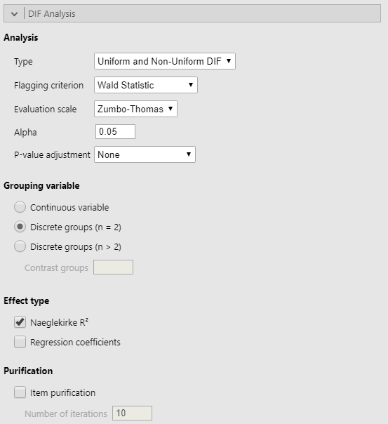
5. Type

    options:
    - Uniform DIF
    - Non-Uniform DIF
    - Uniform and Non-Uniform DIF
    

Type refers to the type of DIF to be assessed for. The default, Uniform and Non-Uniform DIF will check simultaneously for significant main and interaction effects.

6. Flagging Criterion

    options:
      - "Wald"
      - "LRT"
      
      

Flagging Criterion refers to what test should be used in testing for statistical significance of regression coefficients.

7. Evaluation Scale

    options:
          Zumbo-Thomas
          Jodoin-Gierl

Evaluation Scale refers to the classification scheme for DIF effect sizes on the Naeglekirke’s R^2 (Δ R^2) scale.

8. Alpha

Alpha is the desired Type-I error rate for statistical significance tests.

9. P-value Adjustment method

    options: 
        - bonferroni
        - holm
        - hochberg
        - hommel
        - BH
        - BY
        - none
        

P-value Adjustment method is the method of correction for multiple comparisons desired:

The adjustment methods include the Bonferroni correction (“bonferroni”) in which the p-values are multiplied by the number of comparisons. Less conservative corrections are also included by Holm (1979) (“holm”), Hochberg (1988) (“hochberg”), Hommel (1988) (“hommel”), Benjamini & Hochberg (1995) (“BH” or its alias “fdr”), and Benjamini & Yekutieli (2001) (“BY”), respectively. A pass-through option (“none”) is also included. The set of methods are contained in the p.adjust.methods vector for the benefit of methods that need to have the method as an option and pass it on to p.adjust.

The first four methods are designed to give strong control of the family-wise error rate. There seems no reason to use the unmodified Bonferroni correction because it is dominated by Holm’s method, which is also valid under arbitrary assumptions.

Hochberg’s and Hommel’s methods are valid when the hypothesis tests are independent or when they are non-negatively associated (Sarkar, 1998; Sarkar and Chang, 1997). Hommel’s method is more powerful than Hochberg’s, but the difference is usually small and the Hochberg p-values are faster to compute.

The “BH” (aka “fdr”) and “BY” method of Benjamini, Hochberg, and Yekutieli control the false discovery rate, the expected proportion of false discoveries amongst the rejected hypotheses. The false discovery rate is a less stringent condition than the family-wise error rate, so these methods are more powerful than the others.

Note that you can set n larger than length(p) which means the unobserved p-values are assumed to be greater than all the observed p for “bonferroni” and “holm” methods and equal to 1 for the other methods.

10. Grouping variable

    options:
        Continuous variable
        Discrete groups (n = 2)
        Discrete groups (n > 2)
        

Grouping variable specifies how the software should treat the data in the grouping variable. “Discrete Groups (n = 2)”" is the default and will consider the first value in the Grouping Variable column to be the reference group in the logistic regression model. “Discrete Groups (n > 2)”" is to be used when contrasts are to be made between more than two discrete levels. The contrasts must be specified using the Contrast groups argument (see below). “Continuous Groups” is for use when the `Grouping Variable" has not been descritized.

10. Effect type

  options: 
      Naeglekirke R²
      Regression Coefficients

Both Effect type options are True/False and control the display of a DIF results table constructed using their respective effect type.

11. Item Purification

Item purification can be performed by selecting this option. Note that purification is possible only if the test score is considered as the matching criterion.

Purification works as follows: if at least one item is detected as functioning differently at the first step of the process, then the data set of the next step consists in all items that are currently anchor (DIF free) items, plus the tested item (if necessary). The process stops when either two successive applications of the method yield the same classifications of the items (Clauser and Mazor, 1998), or when nrIter iterations are run without obtaining two successive identical classifications. In the latter case a warning message is printed.

12. Number of Iterations type: Number

Number of Iterations is the maximum number of purification iterations to be used if Item Purification is selected.

Type-M Error

Calculating the Type-M error rate for Δ R² is completed via a bootstrapping process which generates an empirical distribution for the Δ R² for each item. The R code for this computation is available below. The variable myBoot contains the empirical distribution, along with the estimate of the standard error.

The design analysis is then carried out according to an extension of the same principles as those laid out in Gelman & Carlin (2014). This analysis by default uses three hypothesized true correlations. The hypothesized true correlations correspond to the level thresholds of the Zumbo-Thomas DIF evaluation scale: 0 (Null/Negligible DIF), 0.13 (Moderate DIF), 0.26 (Large DIF). Those familiar with Type-M error calculations may immediately spot a potential problem with the Null DIF hypothesized true effect. Type-M error is the ratio of the expectation of the observed effect and the hypothesized true effect; in the Null DIF hypothesis, this is 0. In order to bypass this problem, the Null effect is actually hypothesized as being 0 plus 2 times the standard error of the estimated effect size, which is derived during the process of bootstrapping the Δ R² empirical distribution. In effect, this hypothesis is that the unknown true effect is 0 +/- a certain degree of measurement error.

        retroDesign.nagR2 <- function(hypTrueEff, myBoot, alpha, sigOnly) {
          # A matrix for results
          rdRes <- matrix(0, nrow = 1, ncol = 4)
          # The observed Δ R^2
          rdRes[1, 1] <- myBoot$t0
          # se of empirical distribution
          rdRes[1, 4] <- observedSE <- boot.printSE(myBoot)[[3]]
          
          # Observed R^2 is the observed effect
          D <- myBoot$t0
          
          # Empirical cumulative density function on the bootstrapped data
          qUpper <- ecdf(myBoot$t)
          # Either compute Type-M at the provided alpha or for the minimum alpha required for significance
          if (sigOnly) {
            # Quantile matching the upper 1 - alpha in the emp. dist.
            qUpper <- quantile(qUpper,  1 - (alpha))
          } else {
            # Quantile matching the observed value
            qUpper <- boot.qEmp(qUpper, boot.pEmp(qUpper, D))
          }
          
          # shifts the empirical distribution by the difference between the observed effect size and the hypothesized true effect size
          myBoot.Shifted <- ecdf(myBoot$t + hypTrueEff)
          # Empirical observed power
          rdRes[1, 3] <- power <- 1 - myBoot.Shifted(qUpper)
          # typeM error rate via Estimation
          estimate <-
            D + sample(myBoot$t, replace = T, size = 10000)
          significant <- estimate > qUpper
          rdRes[1, 2] <-
            typeMError <- mean(estimate[significant]) / D
          return(rdRes)
        }

The above function is derived from that provided by Gelman & Carlin (2014) in their appendix. The changes are made in order to accomodate the reality that we cannot assume a normal distribution in this case.

Type-S Error

Type-S error is not calculated because it does not align conceptually with the tests being performed in this type of DIF analysis. The Δ R^2 effect size is a meta-statistic, as opposed to a normal measure of effect size like Cohen’s d, and one of the results of this is that Δ R^2 will only be negative in anomalous situations, meaning that there is no meaningful probability of achieving a statistically significant effect in the ‘wrong’ direction.

1. Design Analysis

Design Analysis is a True/False option, defaulted to False. This can be quite computationally intensive. If this option is selected, and then another option is changed, the module will incorporate the change as soon as possible, but several embedded loops mean that there may be a delay before you see the change take effect.

2. Effect type

Effect type may be either Δ Naeglekirke R^2 or Regression Coefficients. This option selects which effect size estimate to perform the design analysis on.

2. Flagged items only

Flagged items only is a True/False option, defaulted to True. This option refers to whether or not you want to perform a post-data design analysis using the same alpha as in the DIF analysis, or using the minimum alpha required for significance for all items.

3. Bootstrap N

Bootstrap N refers to the number of bootstrap replications to be used in creating the empirical distribution for Δ R^2. This is defaulted to 1000 as a balance between computation time and precision. Lower numbers will allow faster exploration, but will provide less stable estimates.

4. Observed Power

Empirical Observed Power is a True/False option, defaulted to False. Toggling this option reveals the column showing the Empirical Observed Power. This is defaulted to False because its interpretation can be confusing, and will not always provide useful information. N.B. The Empirical Observed Power can equal 1 or 0.

5. Hypothesized True Effect Size

Hypothesized True Effect Size is used to perform design analysis using a non-default hypothesized true effect. If left blank, the analysis will be performed at each of the thresholds of the DIF Flag Scale selected above.

1. Item Response Curves based on Logistic Regression type: Variables

Item Respnse Curves is a list of names referring to columns in the data selected for DIF analysis for which logistic regression Item Response Curves should be produced.

Procedure Notes

The descriptive overview provides a textual summary of the whole analysis, including what options were chosen, and documenting any warnings or errors that were encountered during the model fitting process.

DIF Analysis - Results Table

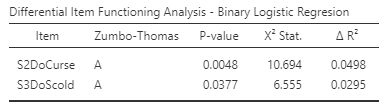
1. Item contains the name of the item under analysis.

2. The second column contains the DIF classification. The legend for classification is at the end of the Procedure Notes.

3. P-value is the p-value of the chi^2 statistic.

4. χ2 Stat. is the chi^2 statistic for the likelihood ratio/Wald test.

5. Δ R^2 is the change in Naeglekirke R^2 between the baseline and full models.

Design Analysis - Results Table

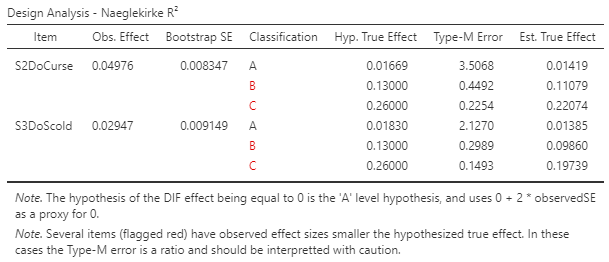
1. Item contains the name of the item under analysis.

2. Obs. Effect is the observed effect size, matching the DIF Results table above.

3. Bootstrap SE is the estimate of the standard error of the effect size estimate, derived during the bootstrap estimation process.

4. Classification is the DIF flag attached to the observed effect size. The legend for classification is at the end of the Procedure Notes.

5. Hyp. True Effect is the hypothesized true effect being used in the Type-M error calculation. The default hypotheses are the thresholds of the three DIF classification levels.

6. Type-M Error is the Type-M error.

7. Est. True Effect is the observed effect divided by the Type-M error. This, in theory, provides a more reasonable/conservative estimate of the true effect, balanced between the theoretical expectation encoded in the hypothesized true effect and the observed effect.

Item Response Curves

The item response curve can be plotted for any item being assessed for DIF. It provides a visual representation of the full model used in the DIF analysis. The different groups are colour coded, with 95% confidence intervals represented by gray shading overlaying each line. In these images the Y-axis is the probability of endorsement (0 to 1), and the X-axis is the range of the matching variable used in the logistic models.